

This chapter demonstrates the use of XSPEC. The brief discussion of data and response files is followed by fully worked examples using real data that include all the screen input and output with a variety of plots. The topics covered are as follows: defining models, fitting data, determining errors, fitting more than one set of data simultaneously, simulating data, and producing plots.
At least two files are necessary for use with XSPEC: a data file and a response file. In some cases, a file containing background may also be used, and, in rare cases, a correction file is needed to adjust the background during fitting. If the response is split between an rmf and an arf then an ancillary response file is also required. However, most of the time the user need only specify the data file, as the names and locations of the correct response and background files should be written in the header of the data file by whatever program created the files.
Our first example uses very old data which is much simpler than more modern observations and so can be used to better illustrate the basics of XSPEC analysis. The 6s X-ray pulsar 1E1048.1–5937 was observed by EXOSAT in June 1985 for 20 ks. In this example, we'll conduct a general investigation of the spectrum from the Medium Energy (ME) instrument, i.e. follow the same sort of steps as the original investigators (Seward, Charles & Smale, 1986). The ME spectrum and corresponding response matrix were obtained from the HEASARC On-line service. Once installed, XSPEC is invoked by typing
%xspec
as in this example:
%xspec
XSPEC version: 12.8.0
Build Date/Time: Thu Nov 29 12:40:42 2012
XSPEC12>data s54405.pha
1 spectrum in use
Spectral Data File: s54405.pha Spectrum 1
Net count rate (cts/s) for Spectrum:1 3.783e+00 +/- 1.367e-01
Assigned to Data Group 1 and Plot Group 1
Noticed Channels: 1-125
Telescope: EXOSAT Instrument: ME Channel Type: PHA
Exposure Time: 2.358e+04 sec
Using fit statistic: chi
Using test statistic: chi
Using Response (RMF) File s54405.rsp for Source 1
The data command tells the program to read the data as well as the response file that is named in the header of the data file. In general, XSPEC commands can be truncated, provided they remain unambiguous. Since the default extension of a data file is .pha, and the abbreviation of data to the first two letters is unambiguous, the above command can be abbreviated to da s54405, if desired. To obtain help on the data command, or on any other command, type help command followed by the name of the command.
One of the first things most users will want to do at this stage—even before fitting models—is to look at their data. The plotting device should be set first, with the command cpd (change plotting device). Here, we use the pgplot X-Window server, /xs.
XSPEC12> cpd /xs
There are more than 50 different things that can be plotted, all related in some way to the data, the model, the fit and the instrument. To see them, type:
XSPEC12> plot ?
plot data/models/fits etc
Syntax: plot commands:
background chain chisq contour counts
data delchi dem emodel eemodel
efficiency eufspec eeufspec foldmodel goodness
icounts insensitivity lcounts ldata margin
model ratio residuals sensitivity sum
ufspec
Multi-panel plots are created by entering multiple commands
e.g. "plot data chisq"
The most fundamental is the data plotted against instrument channel (data); next most fundamental, and more informative, is the data plotted against channel energy. To do this plot, use the XSPEC command setplot energy. Figure A shows the result of the commands:
XSPEC12> setplot energy
XSPEC12> plot data
Note the label on the y-axis. The word “normalized” indicates that this plot has been divided by the value of the EFFAREA keyword in the response file. Usually this is unity so can be ignored. The label also has no cm-2 so the plot is not corrected for the effective area of the detector.
We are now ready to fit the data with a model. Models in XSPEC are specified using the model command, followed by an algebraic expression of a combination of model components. There are two basic kinds of model components: additive, which represent X-Ray sources of different kinds. After being convolved with the instrument response, the components prescribe the number of counts per energy bin (e.g., a bremsstrahlung continuum); and multiplicative models components, which represent phenomena that modify the observed X-Radiation (e.g. reddening or an absorption edge). They apply an energy-dependent multiplicative factor to the source radiation before the result is convolved with the instrumental response.
![]()

Figure A: The result of the command plot data when the data file in question is the EXOSAT ME spectrum of the 6s X-ray pulsar 1E1048.1--5937 available from the HEASARC on-line service
More generally, XSPEC allows three types of modifying components: convolutions and mixing models in addition to the multiplicative type. Since there must be a source, there must be least one additive component in a model, but there is no restriction on the number of modifying components. To see what components are available, just type model :
XSPEC12>model
Additive Models:
apec bapec bbody bbodyrad bexrav bexriv
bkn2pow bknpower bmc bremss bvapec bvvapec
c6mekl c6pmekl c6pvmkl c6vmekl cemekl cevmkl
cflow compLS compPS compST compTT compbb
compmag comptb compth cplinear cutoffpl disk
diskbb diskir diskline diskm disko diskpbb
diskpn eplogpar eqpair eqtherm equil expdec
ezdiskbb gadem gaussian gnei grad grbm
kerrbb kerrd kerrdisk laor laor2 logpar
lorentz meka mekal mkcflow nei npshock
nsa nsagrav nsatmos nsmax nteea nthComp
optxagn optxagnf pegpwrlw pexmon pexrav pexriv
plcabs posm powerlaw pshock raymond redge
refsch sedov sirf smaug srcut sresc
step vapec vbremss vequil vgadem vgnei
vmcflow vmeka vmekal vnei vnpshock vpshock
vraymond vsedov vvapec zbbody zbremss zgauss
zpowerlw
Multiplicative Models:
SSS_ice TBabs TBgrain TBvarabs absori acisabs
cabs constant cyclabs dust edge expabs
expfac gabs highecut hrefl notch pcfabs
phabs plabs pwab recorn redden smedge
spexpcut spline swind1 uvred varabs vphabs
wabs wndabs xion zTBabs zdust zedge
zhighect zigm zpcfabs zphabs zredden zsmdust
zvarabs zvfeabs zvphabs zwabs zwndabs zxipcf
Convolution Models:
cflux gsmooth ireflect kdblur kdblur2 kerrconv
lsmooth partcov rdblur reflect rgsxsrc simpl
zashift zmshift
Mixing Models:
ascac projct suzpsf xmmpsf
Pile-up Models:
pileup
Mixing pile-up Models:
Additional models are available at :
legacy.gsfc.nasa.gov/docs/xanadu/xspec/newmodels.html
For information about a specific component, type help model followed by the name of the component):
XSPEC12>help model apec
Given the quality of our data, as shown by the plot, we'll choose an absorbed power law, specified as follows :
XSPEC12> model phabs(powerlaw)
Or, abbreviating unambiguously:
XSPEC12> mo pha(po)
The user is then prompted for the initial values of the parameters. Entering <return> or / in response to a prompt uses the default values. We could also have set all parameters to their default values by entering /* at the first prompt. As well as the parameter values themselves, users also may specify step sizes and ranges (<value>,<delta>, <min>, <bot>, <top>, and <max values>), but here, we'll enter the defaults:
XSPEC12>mo pha(po)
Input parameter value, delta, min, bot, top, and max values for ...
1 0.001( 0.01) 0 0 100000 1E+06
1:phabs:nH>/*
========================================================================
Model: phabs<1>*powerlaw<2> Source No.: 1 Active/On
Model Model Component Parameter Unit Value
par comp
1 1 phabs nH 10^22 1.00000 +/- 0.0
2 2 powerlaw PhoIndex 1.00000 +/- 0.0
3 2 powerlaw norm 1.00000 +/- 0.0
________________________________________________________________________
Fit statistic : Chi-Squared = 4.864244e+08 using 125 PHA bins.
Test statistic : Chi-Squared = 4.864244e+08 using 125 PHA bins.
Reduced chi-squared = 3.987085e+06 for 122 degrees of freedom
Null hypothesis probability = 0.000000e+00
Current data and model not fit yet.
The current statistic is ![]() and is huge for the initial, default values—mostly
because the power law normalization is two orders of magnitude too large. This
is easily fixed using the renorm command.
and is huge for the initial, default values—mostly
because the power law normalization is two orders of magnitude too large. This
is easily fixed using the renorm command.
XSPEC12> renorm
Fit statistic : Chi-Squared = 852.19 using 125 PHA bins.
Test statistic : Chi-Squared = 852.19 using 125 PHA bins.
Reduced chi-squared = 6.9852 for 122 degrees of freedom
Null hypothesis probability = 7.320332e-110
Current data and model not fit yet.
We are not quite ready to fit the data (and obtain a better ![]() ), because not
all of the 125 PHA bins should be included in the fitting: some are below the
lower discriminator of the instrument and therefore do not contain valid data;
some have imperfect background subtraction at the margins of the pass band; and
some may not contain enough counts for
), because not
all of the 125 PHA bins should be included in the fitting: some are below the
lower discriminator of the instrument and therefore do not contain valid data;
some have imperfect background subtraction at the margins of the pass band; and
some may not contain enough counts for ![]() to be strictly meaningful. To find out which channels to
discard (ignore in XSPEC terminology), consult mission-specific
documentation that will include information about discriminator settings,
background subtraction problems and other issues. For the mature missions in
the HEASARC archives, this information already has been encoded in the headers
of the spectral files as a list of “bad” channels. Simply issue the command:
to be strictly meaningful. To find out which channels to
discard (ignore in XSPEC terminology), consult mission-specific
documentation that will include information about discriminator settings,
background subtraction problems and other issues. For the mature missions in
the HEASARC archives, this information already has been encoded in the headers
of the spectral files as a list of “bad” channels. Simply issue the command:
XSPEC12> ignore bad
ignore: 40 channels ignored from source number 1
Fit statistic : Chi-Squared = 799.74 using 85 PHA bins.
Test statistic : Chi-Squared = 799.74 using 85 PHA bins.
Reduced chi-squared = 9.7529 for 82 degrees of freedom
Null hypothesis probability = 3.545928e-118
Current data and model not fit yet.
XSPEC12> plot ldata chi

Figure B: The result of the command plot ldata chi after the command ignore bad on the EXOSAT ME spectrum 1E1048.1–5937
Giving two options for the plot command generates a plot
with vertically stacked windows. Up to six options can be given to the plot
command at a time. Forty channels were rejected because they were flagged as
bad—but do we need to ignore any more? Figure B shows the result of plotting
the data and the model (in the upper window) and the contributions to ![]() (in the lower
window). We see that above about 15 keV the S/N becomes small. We also see,
comparing Figure B with Figure A, which bad channels were ignored. Although
visual inspection is not the most rigorous method for deciding which channels
to ignore (more on this subject later), it's good enough for now, and will at
least prevent us from getting grossly misleading results from the fitting. To
ignore energies above 15 keV:
(in the lower
window). We see that above about 15 keV the S/N becomes small. We also see,
comparing Figure B with Figure A, which bad channels were ignored. Although
visual inspection is not the most rigorous method for deciding which channels
to ignore (more on this subject later), it's good enough for now, and will at
least prevent us from getting grossly misleading results from the fitting. To
ignore energies above 15 keV:
XSPEC12> ignore 15.0-**
78 channels (48-125) ignored in spectrum # 1
Fit statistic : Chi-Squared = 721.57 using 45 PHA bins.
Test statistic : Chi-Squared = 721.57 using 45 PHA bins.
Reduced chi-squared = 17.180 for 42 degrees of freedom
Null hypothesis probability = 1.250565e-124
Current data and model not fit yet.
If the ignore command is handed a real number it assumes energy in keV while if it is handed an integer it will assume channel number. The “**” just means the highest energy. Starting a range with “**” means the lowest energy. The inverse of ignore is notice, which has the same syntax.
We are now ready to fit the data. Fitting is initiated by
the command fit. As the fit proceeds, the screen displays the status of
the fit for each iteration until either the fit converges to the minimum ![]() , or we are
asked whether the fit is to go through another set of iterations to find the
minimum. The default number of iterations before prompting is ten.
, or we are
asked whether the fit is to go through another set of iterations to find the
minimum. The default number of iterations before prompting is ten.
XSPEC12>fit
Chi-Squared |beta|/N Lvl 1:nH 2:PhoIndex 3:norm
721.533 1.01892e-10 -3 1.00000 1.00000 0.00242602
471.551 150.854 -4 0.152441 1.67440 0.00415548
367.421 60807.7 -3 0.308661 2.31822 0.00958061
53.6787 25662.3 -4 0.503525 2.14501 0.0121712
43.8123 4706.76 -5 0.549824 2.23901 0.0130837
43.802 118.915 -6 0.538696 2.23676 0.0130385
43.802 0.422329 -7 0.537843 2.23646 0.0130320
========================================
Variances and Principal Axes
1 2 3
4.7883E-08| -0.0025 -0.0151 0.9999
8.6821E-02| -0.9153 -0.4026 -0.0084
2.2915E-03| -0.4027 0.9153 0.0128
----------------------------------------
====================================
Covariance Matrix
1 2 3
7.312e-02 3.115e-02 6.564e-04
3.115e-02 1.599e-02 3.207e-04
6.564e-04 3.207e-04 6.561e-06
------------------------------------
========================================================================
Model phabs<1>*powerlaw<2> Source No.: 1 Active/On
Model Model Component Parameter Unit Value
par comp
1 1 phabs nH 10^22 0.537843 +/- 0.270399
2 2 powerlaw PhoIndex 2.23646 +/- 0.126455
3 2 powerlaw norm 1.30320E-02 +/- 2.56146E-03
________________________________________________________________________
Fit statistic : Chi-Squared = 43.80 using 45 PHA bins.
Test statistic : Chi-Squared = 43.80 using 45 PHA bins.
Reduced chi-squared = 1.043 for 42 degrees of freedom
Null hypothesis probability = 3.949507e-01
There is a fair amount of information here so we will unpack it a bit at a time. One line is written out after each fit iteration. The columns labeled Chi-Squared and Parameters are obvious. The other two provide additional information on fit convergence. At each step in the fit a numerical derivative of the statistic with respect to the parameters is calculated. We call the vector of these derivatives beta. At the best-fit the norm of beta should be zero so we write out |beta| divided by the number of parameters as a check. The actual default convergence criterion is when the fit statistic does not change significantly between iterations so it is possible for the fit to end while |beta| is still significantly different from zero. The |beta|/N column helps us spot this case. The Lvl column also indicates how the fit is converging and should generally decrease. Note that on the first iteration only the powerlaw norm is varied. While not necessary this simple model, for more complicated models only varying the norms on the first iteration helps the fit proper get started in a reasonable region of parameter space.
At the end of the fit XSPEC writes out the Variances and Principal Axes and Covariance Matrix sections. These are both based on the second derivatives of the statistic with respect to the parameters. Generally, the larger these second derivatives, the better determined the parameter (think of the case of a parabola in 1-D). The Covariance Matrix is the inverse of the matrix of second derivatives. The Variances and Principal Axes section is based on an eigenvector decomposition of the matrix of second derivatives and indicates which parameters are correlated. We can see in this case that the first eigenvector depends almost entirely on the powerlaw norm while the other two are combinations of the nH and powerlaw PhoIndex. This tells us that the norm is independent but the other two parameters are correlated.
The next section shows the best-fit parameters and error estimates. The latter are just the square roots of the diagonal elements of the covariance matrix so implicitly assume that the parameter space is multidimensional Gaussian with all parameters independent. We already know in this case that the parameters are not independent so these error estimates should only be considered guidelines to help us determine the true errors later.
The final section shows the statistic values at the end of
the fit. XSPEC defines a fit statistic, used to determine the best-fit
parameters and errors, and test statistic, used to decide whether this model
and parameters provide a good fit to the data. By default, both statistics are ![]() . When the test
statistic is
. When the test
statistic is ![]() we can also
calculate the reduced
we can also
calculate the reduced ![]() and
the null hypothesis probability. This latter is the probability of getting a
value of
and
the null hypothesis probability. This latter is the probability of getting a
value of ![]() as large or
larger than observed if the model is correct. If this probability is small then
the model is not a good fit. The null hypothesis probability can be calculated
analytically for
as large or
larger than observed if the model is correct. If this probability is small then
the model is not a good fit. The null hypothesis probability can be calculated
analytically for ![]() but
not for some other test statistics so XSPEC provides another way of determining
the meaning of the statistic value. The goodness command performs
simulations of the data based on the current model and parameters and compares
the statistic values calculated with that for the real data. If the observed
statistic is larger than the values for the simulated data this implies that
the real data do not come from the model. To see how this works we will use the
command for this case (where it is not necessary)
but
not for some other test statistics so XSPEC provides another way of determining
the meaning of the statistic value. The goodness command performs
simulations of the data based on the current model and parameters and compares
the statistic values calculated with that for the real data. If the observed
statistic is larger than the values for the simulated data this implies that
the real data do not come from the model. To see how this works we will use the
command for this case (where it is not necessary)
XSPEC12>goodness 1000
47.40% of realizations are < best fit statistic 43.80 (nosim)
XSPEC12>plot goodness
Approximately
half of the simulations give a statistic value less than that observed,
consistent with this being a good fit. Figure C shows a histogram of the ![]() values from
the simulations with the observed value shown by the vertical dotted line.
values from
the simulations with the observed value shown by the vertical dotted line.
So the statistic implies the fit is good but it is still always a good idea to look at the data and residuals to check for any systematic differences that may not be caught by the test. To see the fit and the residuals, we produce figure D using the command
XSPEC12>plot data resid

Figure C: The result of the command plot goodness. The histogram shows the fraction of simulations with a given value of the statistic and the dotted line marks that for the observed data. There is no reason to reject the model.
Now that we think we have the correct model we need to determine how well the parameters are determined. The screen output at the end of the fit shows the best-fitting parameter values, as well as approximations to their errors. These errors should be regarded as indications of the uncertainties in the parameters and should not be quoted in publications. The true errors, i.e. the confidence ranges, are obtained using the error command. We want to run error on all three parameters which is an intrinsically parallel operation so we can use XSPEC’s support for multiple cores and run the error estimations in parallel:
XSPEC12>parallel error 3
XSPEC12>error 1 2 3
Parameter Confidence Range (2.706)
1 0.107599 1.00722 (-0.430244,0.469381)
2 2.03775 2.44916 (-0.198717,0.2127)
3 0.00954178 0.0181617 (-0.00349017,0.00512978)
Here, the numbers 1, 2, 3 refer to the parameter numbers in
the Model par
column of the output at the end of the fit. For the first parameter, the column
of absorbing hydrogen atoms, the 90% confidence range is ![]() .
This corresponds to an excursion in
.
This corresponds to an excursion in ![]() of
2.706. The reason these “better” errors are not given automatically as part of
the fit output is that they entail further fitting. When the model is
simple, this does not require much CPU, but for complicated models the extra
time can be considerable. The error for each parameter is determined allowing
the other two parameters to vary freely. If the parameters are uncorrelated
this is all the information we need to know. However, we have an indication
from the covariance matrix at the
of
2.706. The reason these “better” errors are not given automatically as part of
the fit output is that they entail further fitting. When the model is
simple, this does not require much CPU, but for complicated models the extra
time can be considerable. The error for each parameter is determined allowing
the other two parameters to vary freely. If the parameters are uncorrelated
this is all the information we need to know. However, we have an indication
from the covariance matrix at the

Figure D: The result of the command plot data resid with: the ME data file from
1E1048.1—5937; “bad” and negative channels ignored; the best-fitting absorbed
power-law model; the residuals of the fit.
end of the fit that the column and photon index are correlated. To investigate this further we can use the command steppar to run a grid over these two parameters:
XSPEC12>steppar 1 0.0 1.5 25 2 1.5 3.0 25
Chi-Squared Delta nH PhoIndex
Chi-Squared 1 2
162.65 118.84 0 0 0 1.5
171.59 127.79 1 0.06 0 1.5
180.87 137.06 2 0.12 0 1.5
190.44 146.64 3 0.18 0 1.5
200.29 156.49 4 0.24 0 1.5
. . . . . . .
316.02 272.22 4 0.24 25 3
334.68 290.88 3 0.18 25 3
354.2 310.4 2 0.12 25 3
374.62 330.82 1 0.06 25 3
395.94 352.14 0 0 25 3
and make the contour plot shown in figure E using:
XSPEC12>plot contour
What else can we do with the fit? One thing is to derive the flux of the model. The data by themselves only give the instrument-dependent count rate. The model, on the other hand, is an estimate of the true spectrum emitted. In XSPEC, the model is defined in physical units
Figure E: The result of the command plot contour. The contours shown are for one, two and three sigma. The cross marks the best-fit position.
independent of the instrument. The command flux integrates the current model over the range specified by the user:
XSPEC12> flux 2 10
Model Flux 0.003539 photons (2.2321e-11 ergs/cm^2/s) range (2.0000 - 10.000 keV)
Here we have chosen the standard X-ray range of 2—10 keV and find that the energy flux is 2.2x10⁻¹¹ erg/cm2/s. Note that flux will integrate only within the energy range of the current response matrix. If the model flux outside this range is desired—in effect, an extrapolation beyond the data---then the command energies should be used. This command defines a set of energies on which the model will be calculated. The resulting model is then remapped onto the response energies for convolution with the response matrix. For example, if we want to know the flux of our model in the ROSAT PSPC band of 0.2—2 keV, we enter:
XSPEC12>energies extend low 0.2 100
Models will use response energies extended to:
Low: 0.2 in 100 log bins
Fit statistic : Chi-Squared = 43.80 using 45 PHA bins.
Test statistic : Chi-Squared = 43.80 using 45 PHA bins.
Reduced chi-squared = 1.043 for 42 degrees of freedom
Null hypothesis probability = 3.949504e-01
Current data and model not fit yet.
XSPEC12>flux 0.2 2.
Model Flux 0.004352 photons (8.847e-12 ergs/cm^2/s) range (0.20000 - 2.0000 keV)
The energy flux, at 8.8x10⁻¹² ergs/cm2/s is lower in this band but the photon flux is higher. The model energies can be reset to the response energies using energies reset.
Calculating the flux is not usually enough, we want its uncertainty as well. The best way to do this is to use the cflux model. Suppose further that what we really want is the flux without the absorption then we include the new cflux model by:
XSPEC12>editmod pha*cflux(pow)
Input parameter value, delta, min, bot, top, and max values for ...
0.5 -0.1( 0.005) 0 0 1e+06 1e+06
2:cflux:Emin>0.2
10 -0.1( 0.1) 0 0 1e+06 1e+06
3:cflux:Emax>2.0
-12 0.01( 0.12) -100 -100 100 100
4:cflux:lg10Flux>-10.3
Fit statistic : Chi-Squared = 3459.85 using 45 PHA bins.
Test statistic : Chi-Squared = 3459.85 using 45 PHA bins.
Reduced chi-squared = 84.3867 for 41 degrees of freedom
Null hypothesis probability = 0.000000e+00
Current data and model not fit yet.
========================================================================
Model phabs<1>*cflux<2>*powerlaw<3> Source No.: 1 Active/On
Model Model Component Parameter Unit Value
par comp
1 1 phabs nH 10^22 0.537843 +/- 0.270399
2 2 cflux Emin keV 0.200000 frozen
3 2 cflux Emax keV 2.00000 frozen
4 2 cflux lg10Flux cgs -10.3000 +/- 0.0
5 3 powerlaw PhoIndex 2.23646 +/- 0.126455
6 3 powerlaw norm 1.30320E-02 +/- 2.56146E-03
________________________________________________________________________
The Emin and Emax parameters are set to the energy range over which we want the flux to be calculated. We also have to fix the norm of the powerlaw because the normalization of the model will now be determined by the lg10Flux parameter. This is done using the freeze command:
XSPEC12>freeze 6
We now run fit to get the best-fit value of lg10Flux as -10.2787 then:
XSPEC12>error 4
Parameter Confidence Range (2.706)
4 -10.4574 -10.0796 (-0.178807,0.199057)
for a 90% confidence range on the 0.2—2 keV unabsorbed flux of 3.49x10⁻¹¹ – 8.33x10⁻¹¹ ergs/cm2/s.
The fit, as we've remarked, is good, and the parameters are constrained. But unless the purpose of our investigation is merely to measure a photon index, it's a good idea to check whether alternative models can fit the data just as well. We also should derive upper limits to components such as iron emission lines and additional continua, which, although not evident in the data nor required for a good fit, are nevertheless important to constrain. First, let's try an absorbed black body:
XSPEC12>mo pha(bb)
Input parameter value, delta, min, bot, top, and max values for ...
1 0.001( 0.01) 0 0 100000 1e+06
1:phabs:nH>/*
========================================================================
Model phabs<1>*bbody<2> Source No.: 1 Active/On
Model Model Component Parameter Unit Value
par comp
1 1 phabs nH 10^22 1.00000 +/- 0.0
2 2 bbody kT keV 3.00000 +/- 0.0
3 2 bbody norm 1.00000 +/- 0.0
________________________________________________________________________
Fit statistic : Chi-Squared = 3.377094e+09 using 45 PHA bins.
Test statistic : Chi-Squared = 3.377094e+09 using 45 PHA bins.
Reduced chi-squared = 8.040700e+07 for 42 degrees of freedom
Null hypothesis probability = 0.000000e+00
Current data and model not fit yet.
XSPEC12>fit
Parameters
Chi-Squared |beta|/N Lvl 1:nH 2:kT 3:norm
1602.34 3.49871e-11 -3 1.00000 3.00000 0.000767254
1535.61 63.3168 0 0.334306 3.01647 0.000673086
1523.48 112166 0 0.157481 2.96616 0.000613283
1491.74 170832 0 0.0668722 2.87681 0.000570110
1444.73 204639 0 0.0228475 2.76753 0.000535213
1387.84 226852 0 0.00205203 2.64901 0.000504579
1325.6 243760 0 0.000843912 2.52648 0.000476503
1256.04 258202 0 0.000287666 2.40140 0.000450137
1179.2 271528 0 3.10806e-05 2.27482 0.000425541
1083.47 283137 0 7.99181e-06 2.13278 0.000401083
Number of trials exceeded: continue fitting? Y
...
...
123.773 25.397 -8 1.87147e-08 0.890295 0.000278599
Number of trials exceeded: continue fitting?
***Warning: Zero alpha-matrix diagonal element for parameter 1
Parameter 1 is pegged at 1.87147e-08 due to zero or negative pivot element, likely
caused by the fit being insensitive to the parameter.
123.773 1.92501 -3 1.87147e-08 0.890205 0.000278596
==============================
Variances and Principal Axes
2 3
2.8677E-04| -1.0000 -0.0000
2.2370E-11| 0.0000 -1.0000
------------------------------
========================
Covariance Matrix
1 2
2.868e-04 9.336e-09
9.336e-09 2.267e-11
------------------------
========================================================================
Model phabs<1>*bbody<2> Source No.: 1 Active/On
Model Model Component Parameter Unit Value
par comp
1 1 phabs nH 10^22 1.87147E-08 +/- -1.00000
2 2 bbody kT keV 0.890205 +/- 1.69343E-02
3 2 bbody norm 2.78596E-04 +/- 4.76176E-06
________________________________________________________________________
Fit statistic : Chi-Squared = 123.77 using 45 PHA bins.
Test statistic : Chi-Squared = 123.77 using 45 PHA bins.
Reduced chi-squared = 2.9470 for 42 degrees of freedom
Null hypothesis probability = 5.417115e-10
Note that after each set of 10 iterations you are asked whether you want to continue. Replying no at these prompts is a good idea if the fit is not converging quickly. Conversely, to avoid having to keep answering the question, i.e., to increase the number of iterations before the prompting question appears, begin the fit with, say fit 100. This command will put the fit through 100 iterations before pausing. To automatically answer yes to all such questions use the command query yes.
Note that the fit has written out a warning about the first parameter and its estimated error is written as -1. This indicates that the fit is unable to constrain the parameter and it should be considered indeterminate. This usually indicates that the model is not appropriate. One thing to check in this case is that the model component has any contribution within the energy range being calculated. Plotting the data and residuals again we obtain Figure F.
The black body fit is obviously not a good one. Not only is ![]() large, but the
best-fitting NH is indeterminate. Inspection of the residuals
confirms this: the pronounced wave-like shape is indicative of a bad choice of
overall continuum.
large, but the
best-fitting NH is indeterminate. Inspection of the residuals
confirms this: the pronounced wave-like shape is indicative of a bad choice of
overall continuum.
Let's try thermal bremsstrahlung next:
XSPEC12>mo pha(br)
Input parameter value, delta, min, bot, top, and max values for ...
1 0.001( 0.01) 0 0 100000 1e+06
1:phabs:nH>/*
 |
Figure F: As for Figure D, but the model is the best-fitting absorbed black body. Note the wave-like shape of the residuals which indicates how poor the fit is, i.e. that the continuum is obviously not a black body.
========================================================================
Model phabs<1>*bremss<2> Source No.: 1 Active/On
Model Model Component Parameter Unit Value
par comp
1 1 phabs nH 10^22 1.00000 +/- 0.0
2 2 bremss kT keV 7.00000 +/- 0.0
3 2 b
remss norm 1.00000 +/- 0.0
________________________________________________________________________
Fit statistic : Chi-Squared = 4.534834e+07 using 45 PHA bins.
Test statistic : Chi-Squared = 4.534834e+07 using 45 PHA bins.
Reduced chi-squared = 1.079722e+06 for 42 degrees of freedom
Null hypothesis probability = 0.000000e+00
Current data and model not fit yet.
XSPEC12>fit
Parameters
Chi-Squared |beta|/N Lvl 1:nH 2:kT 3:norm
156.921 6.92228e-11 -3 1.00000 7.00000 0.00863005
106.765 24.2507 -4 0.264912 6.25747 0.00718902
...
...
40.0331 190.876 0 8.46112e-05 5.28741 0.00831314
========================================
Variances and Principal Axes
1 2 3
1.9514E-08| -0.0016 0.0007 1.0000
1.1574E-02| 0.9738 0.2272 0.0014
5.3111E-01| 0.2272 -0.9738 0.0011
----------------------------------------
====================================
Covariance Matrix
1 2 3
3.839e-02 -1.150e-01 1.427e-04
-1.150e-01 5.043e-01 -5.396e-04
1.427e-04 -5.396e-04 6.287e-07
------------------------------------
========================================================================
Model phabs<1>*bremss<2> Source No.: 1 Active/On
Model Model Component Parameter Unit Value
par comp
1 1 phabs nH 10^22 8.46112E-05 +/- 0.195940
2 2 bremss kT keV 5.28741 +/- 0.710133
3 2 bremss norm 8.31314E-03 +/- 7.92890E-04
________________________________________________________________________
Fit statistic : Chi-Squared = 40.03 using 45 PHA bins.
Test statistic : Chi-Squared = 40.03 using 45 PHA bins.
Reduced chi-squared = 0.9532 for 42 degrees of freedom
Null hypothesis probability = 5.576222e-01
Bremsstrahlung is a better fit than the black body—and is as good as the power law—although it shares the low NH. With two good fits, the power law and the bremsstrahlung, it's time to scrutinize their parameters in more detail.
First, we reset our fit to the powerlaw (output omitted):
XSPEC12>mo pha(po)
From the EXOSAT database on HEASARC, we know that the
target in question, 1E1048.1--5937, has a Galactic latitude of ![]() , i.e., almost on
the plane of the Galaxy. In fact, the database also provides the value of the
Galactic NH based on 21-cm radio observations. At 4x10²²
cm-2, it is higher than the 90 percent-confidence upper limit from
the power-law fit. Perhaps, then, the power-law fit is not so good after all.
What we can do is fix (freeze in XSPEC terminology) the value of NH
at the Galactic value and refit the power law. Although we won't get a good
fit, the shape of the residuals might give us a clue to what is missing. To
freeze a parameter in XSPEC, use the command freeze followed by the
parameter number, like this:
, i.e., almost on
the plane of the Galaxy. In fact, the database also provides the value of the
Galactic NH based on 21-cm radio observations. At 4x10²²
cm-2, it is higher than the 90 percent-confidence upper limit from
the power-law fit. Perhaps, then, the power-law fit is not so good after all.
What we can do is fix (freeze in XSPEC terminology) the value of NH
at the Galactic value and refit the power law. Although we won't get a good
fit, the shape of the residuals might give us a clue to what is missing. To
freeze a parameter in XSPEC, use the command freeze followed by the
parameter number, like this:
XSPEC12> freeze 1
The inverse of freeze is thaw:
XSPEC12> thaw 1
Figure G: As for Figure D & F, but the model is the best-fitting power law with the absorption fixed at the Galactic value. Under the assumptions that the absorption really is the same as the 21-cm value and that the continuum really is a power law, this plot provides some indication of what other components might be added to the model to improve the fit.
Alternatively, parameters can be frozen using the newpar command, which
allows all the quantities associated with a parameter to be changed. We can
flip between frozen and thawed states by entering 0 after the new parameter
value. In our case, we want NH frozen at 4x1022 cm-2,
so we go back to the power law best fit and do the following :
XSPEC12>newpar 1
Current value, delta, min, bot, top, and max values
0.537843 0.001(0.00537843) 0 0 100000 1e+06
1:phabs[1]:nH:1>4,0
Fit statistic : Chi-Squared = 823.34 using 45 PHA bins.
Test statistic : Chi-Squared = 823.34 using 45 PHA bins.
Reduced chi-squared = 19.148 for 43 degrees of freedom
Null hypothesis probability = 6.151383e-145
Current data and model not fit yet.
The same result can be obtained by putting everything onto the command line, i.e., newpar 1 4, 0, or by issuing the two commands, newpar 1 4 followed by freeze 1. Now, if we fit and plot again, we get the following model (Fig. G).
XSPEC12>fit
...
========================================================================
Model phabs<1>*powerlaw<2> Source No.: 1 Active/On
Model Model Component Parameter Unit Value
par comp
1 1 phabs nH 10^22 4.00000 frozen
2 2 powerlaw PhoIndex 3.59784 +/- 6.76670E-02
3 2 powerlaw norm 0.116579 +/- 9.43208E-03
________________________________________________________________________
Fit statistic : Chi-Squared = 136.04 using 45 PHA bins.
The fit is not good. In Figure G we can see why: there appears to be a surplus of softer photons, perhaps indicating a second continuum component. To investigate this possibility we can add a component to our model. The editmod command lets us do this without having to respecify the model from scratch. Here, we'll add a black body component.
XSPEC12>editmod pha(po+bb)
Input parameter value, delta, min, bot, top, and max values for ...
3 0.01( 0.03) 0.0001 0.01 100 200
4:bbody:kT>2,0
1 0.01( 0.01) 0 0 1e+24 1e+24
5:bbody:norm>1e-5
Fit statistic : Chi-Squared = 132.76 using 45 PHA bins.
Test statistic : Chi-Squared = 132.76 using 45 PHA bins.
Reduced chi-squared = 3.1610 for 42 degrees of freedom
Null hypothesis probability = 2.387580e-11
Current data and model not fit yet.
========================================================================
Model phabs<1>(powerlaw<2> + bbody<3>) Source No.: 1 Active/On
Model Model Component Parameter Unit Value
par comp
1 1 phabs nH 10^22 4.00000 frozen
2 2 powerlaw PhoIndex 3.59784 +/- 6.76670E-02
3 2 powerlaw norm 0.116579 +/- 9.43208E-03
4 3 bbody kT keV 2.00000 frozen
5 3 bbody norm 1.00000E-05 +/- 0.0
________________________________________________________________________
Notice that in specifying the initial values of the black body, we have frozen kT at 2 keV (the canonical temperature for nuclear burning on the surface of a neutron star in a low-mass X-ray binary) and started the normalization at zero. Without these measures, the fit might “lose its way”. Now, if we fit, we get (not showing all the iterations this time):
========================================================================
Model phabs<1>(powerlaw<2> + bbody<3>) Source No.: 1 Active/On
Model Model Component Parameter Unit Value
par comp
1 1 phabs nH 10^22 4.00000 frozen
2 2 powerlaw PhoIndex 4.89584 +/- 0.158997
3 2 powerlaw norm 0.365230 +/- 5.25376E-02
Figure H: The result of the command plot model in the case of the ME data file from 1E1048.1—5937. Here, the model is the best-fitting combination of power law, black body and fixed Galactic absorption. The three lines show the two continuum components (absorbed to the same degree) and their sum.
4 3 bbody kT keV 2.00000 frozen
5 3 bbody norm 2.29697E-04 +/- 2.04095E-05
________________________________________________________________________
Fit statistic : Chi-Squared = 69.53 using 45 PHA bins.
The fit is better than the one with just a power law and the fixed Galactic column, but it is still not good. Thawing the black body temperature and fitting does of course improve the fit but the powerl law index becomes even steeper. Looking at this odd model with the command
XSPEC12> plot model
We see, in Figure H, that the black body and the power law have changed places, in that the power law provides the soft photons required by the high absorption, while the black body provides the harder photons. We could continue to search for a plausible, well-fitting model, but the data, with their limited signal-to-noise and energy resolution, probably don't warrant it (the original investigators published only the power law fit).
There is, however, one final, useful thing to do with the data: derive an upper limit to the presence of a fluorescent iron emission line. First we delete the black body component using delcomp then thaw NH and refit to recover our original best fit. Now, we add a gaussian emission line of fixed energy and width then fit to get:
========================================================================
Model phabs<1>(powerlaw<2> + gaussian<3>) Source No.: 1 Active/On
Model Model Component Parameter Unit Value
par comp
1 1 phabs nH 10^22 0.753989 +/- 0.320344
2 2 powerlaw PhoIndex 2.38165 +/- 0.166973
3 2 powerlaw norm 1.59131E-02 +/- 3.94947E-03
4 3 gaussian LineE keV 6.40000 frozen
5 3 gaussian Sigma keV 0.100000 frozen
6 3 gaussian norm 7.47368E-05 +/- 4.74253E-05
________________________________________________________________________
The energy and width have to be frozen because, in the absence of an obvious line in the data, the fit would be completely unable to converge on meaningful values. Besides, our aim is to see how bright a line at 6.4 keV can be and still not ruin the fit. To do this, we fit first and then use the error command to derive the maximum allowable iron line normalization. We then set the normalization at this maximum value with newpar and, finally, derive the equivalent width using the eqwidth command. That is:
XSPEC12>err 6
Parameter Confidence Range (2.706)
***Warning: Parameter pegged at hard limit: 0
6 0 0.000151164 (-7.476e-05,7.64036e-05)
XSPEC12>new 6 0.000151164
Fit statistic : Chi-Squared = 46.03 using 45 PHA bins.
Test statistic : Chi-Squared = 46.03 using 45 PHA bins.
Reduced chi-squared = 1.123 for 41 degrees of freedom
Null hypothesis probability = 2.717072e-01
Current data and model not fit yet.
XSPEC12>eqwidth 3
Data group number: 1
Additive group equiv width for Component 3: 0.784168 keV
Things to note:
The true minimum value of the gaussian normalization is less
than zero, but the error command stopped searching for a ![]() of
2.706 when the minimum value hit zero, the “hard” lower limit of the parameter.
Hard limits can be adjusted with the newpar command, and they correspond
to the quantities min
and max
associated with the parameter values.
of
2.706 when the minimum value hit zero, the “hard” lower limit of the parameter.
Hard limits can be adjusted with the newpar command, and they correspond
to the quantities min
and max
associated with the parameter values.
The command eqwidth takes the component number as its argument.
The upper limit on the equivalent width of a 6.4 keV emission line is high (784 eV)!
XSPEC has the very useful facility of allowing models to be fitted simultaneously to more than one data file. It is even possible to group files together and to fit different models simultaneously. Reasons for fitting in this manner include:
The same target is observed at several epochs but, although the source stays constant, the response matrix has changed. When this happens, the data files cannot be added together; they have to be fitted separately. Fitting the data files simultaneously yields tighter constraints.
The same target is observed with different instruments. All the instruments on Suzaku, for example, observe in the same direction simultaneously. As far as XSPEC is concerned, this is just like the previous case: two data files with two responses fitted simultaneously with the same model.
Different targets are observed, but the user wants to fit the same model to each data file with some parameters shared and some allowed to vary separately. For example, if we have a series of spectra from a variable AGN, we might want to fit them simultaneously with a model that has the same, common photon index but separately vary the normalization and absorption.
Other scenarios are possible---the important thing is to recognize the flexibility of XSPEC in this regard.
As an example we will look at a case of fitting the same model to two different data files but where not all the parameters are identical. Again, this is an older dataset that provides a simpler illustration than more modern data. The massive X-ray binary Centaurus X-3 was observed with the LAC on Ginga in 1989. Its flux level before eclipse was much lower than the level after eclipse. Here, we'll use XSPEC to see whether spectra from these two phases can be fitted with the same model, which differs only in the amount of absorption. This kind of fitting relies on introducing an extra dimension, the group, to the indexing of the data files. The files in each group share the same model but not necessarily the same parameter values, which may be shared as common to all the groups or varied separately from group to group. Although each group may contain more than one file, there is only one file in each of the two groups in this example. Groups are specified with the data command, with the group number preceding the file number, like this:
XSPEC12>data 1:1 losum 2:2 hisum
2 spectra in use
Spectral Data File: losum.pha Spectrum 1
Net count rate (cts/s) for Spectrum:1 1.401e+02 +/- 3.549e-01
Assigned to Data Group 1 and Plot Group 1
Noticed Channels: 1-48
Telescope: GINGA Instrument: LAC Channel Type: PHA
Exposure Time: 1 sec
Using fit statistic: chi
Using test statistic: chi
Using Response (RMF) File ginga_lac.rsp for Source 1
Spectral Data File: hisum.pha Spectrum 2
Net count rate (cts/s) for Spectrum:2 1.371e+03 +/- 3.123e+00
Assigned to Data Group 2 and Plot Group 2
Noticed Channels: 1-48
Telescope: GINGA Instrument: LAC Channel Type: PHA
Exposure Time: 1 sec
Using fit statistic: chi
Using test statistic: chi
Using Response (RMF) File ginga_lac.rsp for Source 1
Here, the first group makes up the file losum.pha, which contains the spectrum of all the low, pre-eclipse emission. The second group makes up the second file, hisum.pha, which contains all the high, post-eclipse emission. Note that file number is “absolute” in the sense that it is independent of group number. Thus, if there were three files in each of the two groups (lo1.pha, lo2.pha, lo3.pha, hi1.pha, hi2.pha, and hi3.pha, say), rather than one, the six files would be specified as da 1:1 lo1 1:2 lo2 1:3 lo3 2:4 hi1 2:5 hi2 2:6 hi3. The ignore command works on file number, and does not take group number into account. So, to ignore channels 1–3 and 37–48 of both files:
XSPEC12> ignore 1-2:1-3 37-48
The model we'll use at first to fit the two files is an absorbed power law with a high-energy cut-off:
XSPEC12> mo phabs * highecut (po)
After defining the model, we will be prompted for two sets of parameter values, one for the first group of data files (losum.pha), the other for the second group (hisum.pha). Here, we'll enter the absorption column of the first group as 1024 cm–2 and enter the default values for all the other parameters in the first group. Now, when it comes to the second group of parameters, we enter a column of 1022 cm–2 and then enter defaults for the other parameters. The rule being applied here is as follows: to tie parameters in the second group to their equivalents in the first group, take the default when entering the second-group parameters; to allow parameters in the second group to vary independently of their equivalents in the first group, enter different values explicitly:
XSPEC12>mo phabs*highecut(po)
Input parameter value, delta, min, bot, top, and max values for ...
Current: 1 0.001 0 0 1E+05 1E+06
DataGroup 1:phabs:nH>100
Current: 10 0.01 0.0001 0.01 1E+06 1E+06
DataGroup 1:highecut:cutoffE>
Current: 15 0.01 0.0001 0.01 1E+06 1E+06
DataGroup 1:highecut:foldE>
Current: 1 0.01 -3 -2 9 10
DataGroup 1:powerlaw:PhoIndex>
Current: 1 0.01 0 0 1E+24 1E+24
DataGroup 1:powerlaw:norm>
Current: 100 0.001 0 0 1E+05 1E+06
DataGroup 2:phabs:nH>1
Current: 10 0.01 0.0001 0.01 1E+06 1E+06
DataGroup 2:highecut:cutoffE>/*
========================================================================
Model phabs<1>*highecut<2>*powerlaw<3> Source No.: 1 Active/On
Model Model Component Parameter Unit Value
par comp
Data group: 1
1 1 phabs nH 10^22 100.000 +/- 0.0
2 2 highecut cutoffE keV 10.0000 +/- 0.0
3 2 highecut foldE keV 15.0000 +/- 0.0
4 3 powerlaw PhoIndex 1.00000 +/- 0.0
5 3 powerlaw norm 1.00000 +/- 0.0
Data group: 2
6 1 phabs nH 10^22 1.00000 +/- 0.0
7 2 highecut cutoffE keV 10.0000 = 2
8 2 highecut foldE keV 15.0000 = 3
9 3 powerlaw PhoIndex 1.00000 = 4
10 3 powerlaw norm 1.00000 = 5
________________________________________________________________________
Notice how the summary of the model, displayed immediately
above, is different now that we have two groups, as opposed to one (as in all
the previous examples). We can see that of the 10 model parameters, 6 are free
(i.e., 4 of the second group parameters are tied to their equivalents in the
first group). Fitting this model results in a huge ![]() (not shown here), because our assumption that only a
change in absorption can account for the spectral variation before and after
eclipse is clearly wrong. Perhaps scattering also plays a role in reducing the
flux before eclipse. This could be modeled (simply at first) by allowing the
normalization of the power law to be smaller before eclipse than after eclipse.
To decouple tied parameters, we change the parameter value in the second group
to a value—any value—different from that in the first group (changing the value
in the first group has the effect of changing both without decoupling). As
usual, the newpar command is used:
(not shown here), because our assumption that only a
change in absorption can account for the spectral variation before and after
eclipse is clearly wrong. Perhaps scattering also plays a role in reducing the
flux before eclipse. This could be modeled (simply at first) by allowing the
normalization of the power law to be smaller before eclipse than after eclipse.
To decouple tied parameters, we change the parameter value in the second group
to a value—any value—different from that in the first group (changing the value
in the first group has the effect of changing both without decoupling). As
usual, the newpar command is used:
XSPEC12>newpar 10 1
Fit statistic : Chi-Squared = 2.062941e+06 using 66 PHA bins.
Test statistic : Chi-Squared = 2.062941e+06 using 66 PHA bins.
Reduced chi-squared = 34965.10 for 59 degrees of freedom
Null hypothesis probability = 0.000000e+00
Current data and model not fit yet.
XSPEC12>fit
...
========================================================================
Model phabs<1>*highecut<2>*powerlaw<3> Source No.: 1 Active/On
Model Model Component Parameter Unit Value
par comp
Data group: 1
1 1 phabs nH 10^22 20.1531 +/- 0.181904
2 2 highecut cutoffE keV 14.6846 +/- 5.59251E-02
3 2 highecut foldE keV 7.41660 +/- 8.99545E-02
4 3 powerlaw PhoIndex 1.18690 +/- 6.33054E-03
5 3 powerlaw norm 5.88294E-02 +/- 9.30380E-04
Data group: 2
6 1 phabs nH 10^22 1.27002 +/- 3.77708E-02
7 2 highecut cutoffE keV 14.6846 = 2
8 2 highecut foldE keV 7.41660 = 3
9 3 powerlaw PhoIndex 1.18690 = 4
10 3 powerlaw norm 0.312117 +/- 4.49061E-03
________________________________________________________________________
Fit statistic : Chi-Squared = 15423.79 using 66 PHA bins.
After fitting, this decoupling reduces ![]() by a factor of
six to 15,478, but this is still too high. Indeed, this simple attempt to
account for the spectral variability in terms of “blanket” cold absorption and
scattering does not work. More sophisticated models, involving additional
components and partial absorption, should be tried.
by a factor of
six to 15,478, but this is still too high. Indeed, this simple attempt to
account for the spectral variability in terms of “blanket” cold absorption and
scattering does not work. More sophisticated models, involving additional
components and partial absorption, should be tried.
In the previous section we showed how to fit the same model to multiple datasets. We now demonstrate how to fit multiple models, each with their own response, to the same dataset. There are several reasons why this may be useful, for instance:
We are using data from a coded aperture mask. If there are multiple sources in the field they will all contribute to the spectrum from each detector. However, each source may have a different response due to its position.
We are observing an extended source using a telescope whose PSF is large enough that the signal from different regions are mixed together. In this case we will want to analyze spectra from all regions of the source simultaneously with each spectrum having a contribution from the model in other regions.
We wish to model the background spectrum that includes a particle component. The particle background will have a different response from the X-ray background because the particles come from all directions, not just down the telescope.
We will demonstrate the third example here. Suppose we have a model for the background spectrum that requires a different response to that for the source spectrum. Read in the source and background spectra as separate files:
XSPEC12>data 1:1 source.pha 2:2 back.pha
The source and background files have their own response matrices:
XSPEC12>response 1 source.rsp 2 back.rsp
Set up the model for the source. Here we will take the simple case of an absorbed power-law:
XSPEC12>model phabs(pow)
Input parameter value, delta, min, bot, top, and max values for ...
1 0.001( 0.01) 0 0 100000 1e+06
1:data group 1::phabs:nH>
1 0.01( 0.01) -3 -2 9 10
2:data group 1::powerlaw:PhoIndex>
1 0.01( 0.01) 0 0 1e+24 1e+24
3:data group 1::powerlaw:norm>
Input parameter value, delta, min, bot, top, and max values for ...
1 0.001( 0.01) 0 0 100000 1e+06
4:data group 2::phabs:nH>
1 0.01( 0.01) -3 -2 9 10
5:data group 2::powerlaw:PhoIndex>
1 0.01( 0.01) 0 0 1e+24 1e+24
6:data group 2::powerlaw:norm>0 0
Note that we have fixed the normalization of the source model for the background dataset at zero so it doesn't contribute. Now we need to set up the background model for both datasets with its own response matrix.
XSPEC12>response 2:1 back.rsp 2:2 back.rsp
This tells XSPEC that both these datasets have a second model which must be multiplied by the back.rsp response matrix. We now define the background model to be used. In this case take the simple example of a single power-law
XSPEC12>model 2:myback pow
Input parameter value, delta, min, bot, top, and max values for ...
1 0.01( 0.01) -3 -2 9 10
1:myback:data group 1::powerlaw:PhoIndex>
1 0.01( 0.01) 0 0 1e+24 1e+24
2:myback:data group 1::powerlaw:norm>
Input parameter value, delta, min, bot, top, and max values for ...
1 0.01( 0.01) -3 -2 9 10
3:myback:data group 2::powerlaw:PhoIndex>
1 0.01( 0.01) 0 0 1e+24 1e+24
4:myback:data group 2::powerlaw:norm>
We have now set up XSPEC so that the source data is compared to a source model multiplied by the source response plus a background model multiplied by the background response and the background data is compared to the background model multiplied by the background response. The background models fitted to the source and background data are constrained to be the same.
XSPEC12>show param
Parameters defined:
========================================================================
Model phabs<1>*powerlaw<2> Source No.: 1 Active/On
Model Model Component Parameter Unit Value
par comp
Data group: 1
1 1 phabs nH 10^22 1.00000 +/- 0.0
2 2 powerlaw PhoIndex 1.00000 +/- 0.0
3 2 powerlaw norm 1.00000 +/- 0.0
Data group: 2
4 1 phabs nH 10^22 1.00000 = 1
5 2 powerlaw PhoIndex 1.00000 = 2
6 2 powerlaw norm 1.00000 = 3
________________________________________________________________________
========================================================================
Model myback:powerlaw<1> Source No.: 2 Active/On
Model Model Component Parameter Unit Value
par comp
Data group: 1
1 1 powerlaw PhoIndex 1.00000 +/- 0.0
2 1 powerlaw norm 1.00000 +/- 0.0
Data group: 2
3 1 powerlaw PhoIndex 1.00000 = myback:1
4 1 powerlaw norm 1.00000 = myback:2
________________________________________________________________________
It is often the case that the response information is split into an RMF and ARF, where the RMF describes the instrument response and the ARF the telescope effective area. The particle background can then be included by using the RMF but not the ARF:
XSPEC12>data 1:1 source.pha 2:2 back.pha
XSPEC12>response 1 source.rmf 2 source.rmf
XSPEC12>arf 1 source.arf
XSPEC12>response 2:1 source.rmf 2:2 source.rmf
In several cases, analyzing simulated data is a powerful tool to demonstrate feasibility. For example:
To support an observing proposal. That is, to demonstrate what constraints a proposed observation would yield.
To support a hardware proposal. If a response matrix is generated, it can be used to demonstrate what kind of science could be done with a new instrument.
To support a theoretical paper. A theorist could write a paper describing a model, and then show how these model spectra would appear when observed. This, of course, is very like the first case.
Here, we will illustrate the first example. The first step is to define a model on which to base the simulation. The way XSPEC creates simulated data is to take the current model, convolve it with the current response matrix, while adding noise appropriate to the integration time specified. Once created, the simulated data can be analyzed in the same way as real data to derive confidence limits.
Let us suppose that we want to measure the intrinsic absorption of a faint high-redshift source using Chandra. Our model is thus a power-law absorbed both by the local Galactic column and an intrinsic column. First, we set up the model. From the literature we have the Galactic absorption column and redshift so:
XSPEC12>mo pha*zpha(zpo)
Input parameter value, delta, min, bot, top, and max values for ...
1 0.001( 0.01) 0 0 100000 1e+06
1:phabs:nH>0.08
1 0.001( 0.01) 0 0 100000 1e+06
2:zphabs:nH>1.0
0 -0.01( 0.01) -0.999 -0.999 10 10
3:zphabs:Redshift>5.1
1 0.01( 0.01) -3 -2 9 10
4:zpowerlw:PhoIndex>1.7
0 -0.01( 0.01) -0.999 -0.999 10 10
5:zpowerlw:Redshift>5.1
1 0.01( 0.01) 0 0 1e+24 1e+24
6:zpowerlw:norm>
========================================================================
Model phabs<1>*zphabs<2>*zpowerlw<3> Source No.: 1 Active/Off
Model Model Component Parameter Unit Value
par comp
1 1 phabs nH 10^22 8.00000E-02 +/- 0.0
2 2 zphabs nH 10^22 1.00000 +/- 0.0
3 2 zphabs Redshift 5.10000 frozen
4 3 zpowerlw PhoIndex 1.70000 +/- 0.0
5 3 zpowerlw Redshift 5.10000 frozen
6 3 zpowerlw norm 1.00000 +/- 0.0
Now suppose that we know that the observed 0.5—2.5 keV flux is 1.1x10⁻¹³ ergs/cm2/s. We now can derive the correct normalization by using the commands energies, flux and newpar. That is, we'll determine the flux of the model with the normalization of unity. We then work out the new normalization and reset it:
XSPEC12>energies 0.5 2.5 1000
XSPEC12>flux 0.5 2.5
Model Flux 0.052736 photons (1.0017e-10 ergs/cm^2/s) range (0.50000 - 2.5000 keV)
XSPEC12> newpar 6 1.1e-3
3 variable fit parameters
XSPEC12>flux
Model Flux 2.6368e-05 photons (5.0086e-14 ergs/cm^2/s) range (0.50000 - 2.5000 keV)
Here, we have changed the value of the normalization (the fifth parameter) from 1.0 to 1.1x10⁻¹³ / 1.00x10-10 = 1.1x10⁻³ to give the required flux.
The simulation is initiated with the command fakeit. If the argument none is given, we will be prompted for the name of the response matrix. If no argument is given, the current response will be used. We also need to reset the energies command before the fakeit to ensure that the model is calculated on the entire energy range of the response:
XSPEC12>energies reset
XSPEC12>fakeit none
For fake data, file #1 needs response file: aciss_aimpt_cy15.rmf
... and ancillary response file: aciss_aimpt_cy15.arf
There then follows a series of prompts asking the user to specify whether he or she wants counting statistics (yes!), the name of the fake data (file test.fak in our example), and the integration time (40,000 seconds -- the correction norm and background exposure time can be left at their default values).
Use counting statistics in creating fake data? (y):
Input optional fake file prefix:
Fake data file name (aciss_aimpt_cy15.fak): test.fak
Exposure time, correction norm, bkg exposure time (1.00000, 1.00000, 1.00000): 40000.0
No background will be applied to fake spectrum #1
1 spectrum in use
Fit statistic : Chi-Squared = 350.95 using 1024 PHA bins.
***Warning: Chi-square may not be valid due to bins with zero variance
in spectrum number(s): 1
Test statistic : Chi-Squared = 350.95 using 1024 PHA bins.
Reduced chi-squared = 0.34407 for 1020 degrees of freedom
Null hypothesis probability = 1.000000e+00
***Warning: Chi-square may not be valid due to bins with zero variance
in spectrum number(s): 1
Current data and model not fit yet.
The first thing we should note is that the default statistics are not correct for these data. For Poisson data and no background we should cstat for the fit statistic and pchi for the test statistic:
XSPEC12>statistic cstat
Default fit statistic is set to: C-Statistic
This will apply to all current and newly loaded spectra.
Fit statistic : C-Statistic = 513.63 using 1024 PHA bins and 1020 degrees of freedom.
Test statistic : Chi-Squared = 350.95 using 1024 PHA bins.
Reduced chi-squared = 0.34407 for 1020 degrees of freedom
Null hypothesis probability = 1.000000e+00
***Warning: Chi-square may not be valid due to bins with zero variance
in spectrum number(s): 1
Current data and model not fit yet.
XSPEC12>statistic test pchi
Default test statistic is set to: Pearson Chi-Squared
This will apply to all current and newly loaded spectra.
Fit statistic : C-Statistic = 513.63 using 1024 PHA bins and 1020 degrees of freedom.
Test statistic : Pearson Chi-Squared = 639.35 using 1024 PHA bins.
Reduced chi-squared = 0.62682 for 1020 degrees of freedom
Null hypothesis probability = 1.000000e+00
***Warning: Pearson Chi-square may not be valid due to bins with zero model value
in spectrum number(s): 1
Current data and model not fit yet.
As we can see from the warning message we need to ignore some channels where there is no effective response. Looking at a plot of the data and model indicates we should ignore below 0.15 keV and above 10 keV so:
XSPEC12>ignore **-0.15 10.0-**
11 channels (1-11) ignored in spectrum # 1
340 channels (685-1024) ignored in spectrum # 1
Fit statistic : C-Statistic = 510.55 using 673 PHA bins and 669 degrees of freedom.
Test statistic : Pearson Chi-Squared = 635.19 using 673 PHA bins.
Reduced chi-squared = 0.94947 for 669 degrees of freedom
Null hypothesis probability = 8.217205e-01
Current data and model not fit yet.
We assume that the Galactic column is known so freeze the first parameter. We then perform a fit followed by the error command:
XSPEC12> freeze 1
...
XSPEC12>fit
...
XSPEC12>parallel error 3
XSPEC12>err 2 4 6
Parameter Confidence Range ( 2.706)
2 1.16302 5.64805 (-2.00255,2.48247)
4 1.73345 1.95111 (-0.106137,0.111521)
6 0.00126229 0.00221906 (-0.000397759,0.000559019)
Note that our input parameters do not lie within the 90% confidence errors however since this will happen one times in ten (by definition) this should not worry us unduly. For a real observing proposal we would likely repeat this experiment with different input values of the intrinsic absorption to learn how well we could constrain it given a range of possible actual values.
The final results of using XSPEC are usually one or more tables containing confidence ranges and fit statistics, and one or more plots showing the fits themselves. So far, the plots shown have generally used the default settings, but it is possible to edit plots to improve their appearance.
The plotting package used by XSPEC is PGPLOT, which is comprised of a library of low-level tasks. At a higher level is QDP/PLT, the interactive program that forms the interface between the XSPEC user and PGPLOT. QDP/PLT has its own manual; it also comes with on-line help. Here, we show how to make some of the most common modifications to plots.
In this example, we'll take the simulated Chandra spectrum and make a better plot. Figure I shows the basic data and folded model plot. The only additional changes we have made to this plot are to increase the line widths to make them print better. We made this plot as follows:
XSPEC12>setplot energy
XSPEC12>iplot data
PLT>lwidth 3
PLT>lwidth 3 on 1..2
PLT>time off
PLT>hard figi.ps/ps
The first lwidth command increases the line widths on the frame while the second increases it on the data and model. The time off command just removes a username and time stamp from the bottom right of the plot. The hard command makes a “hardcopy”, in this case a PostScript file. Before looking at other PLT commands we can use to modify the plot there is one more thing we can try at the XSPEC level. The current bin sizes are much smaller than the resolution so we may as well combine bins in the plot (but not in the fitting) to make it clearer.
XSPEC12>setplot rebin 100 4
Combines four spectral bins into one. The setplot rebin command combines bins till either a S/N of the first argument is reached or the number of bins in the second argument have been combined. We do an iplot again then do the following modifications:
PLT> viewport 0.2 0.2 0.8 0.7
The first thing we'll do is change the aspect ratio of the box that contains the plot (viewport in QDP terminology). The viewport is defined as the coordinates of the lower left and upper right corners of the page. The units are such that the full width and height of the page are unity. The labels fall outside the viewport, so if the full viewport were specified, only the plot would appear. The default box has a viewport with corners at (0.1, 0.1) and (0.9, 0.9). For our purposes, we want a viewport with corners at (0.2, 0.2) and (0.8, 0.7): with this size and shape, the hardcopy will fit nicely on the page and not have to be reduced for photocopying.
Figure I: The data and folded model for the simulated Chandra ACIS-S spectrum.
Next we want to change some of the labels:
PLT> label top Simulated Spectrum
PLT> label file Chandra ACIS-S
PLT> label y counts s\u-1\d keV\u-1\d
Note the change in the y-axis label is to remove the string “normalized”. The normalization referred to is almost always unity so this label can generally be changed. To get help on a PLT command, just type help followed by the name of the command. Note that PLT commands can be abbreviated, just like XSPEC commands. To see the results of changing the viewport and the labels, just enter the command plot.
The two changes we want to make next are to rescale the axes and to change the y-axis to a logarithmic scale. The commands for these changes also are straightforward: the rescale command takes the minimum and maximum values as its arguments, while the log command takes x or y as arguments:
PLT> rescale x 0.3 6.0
PLT> rescale y 1.0e-4 0.03
PLT> log y
PLT> plot
To revert to a linear scale, use the command log off y. The only remaining extra change is to reduce the size of the characters. This is done using the csize command, which takes the normalization as its argument. One (1) will not change the size, a number less than one will reduce it and a number bigger than one will increase it.
Figure J: A simulated Chandra ACIS-S spectrum produced to show how a plot can be modified by the user.
PLT> csize 0.8
PLT> plot
We make the PostScript file and also save the plot information using the wenv command that, in this case, writes files figj.qdp and figj.pco containing the plot data and commands, respectively.
PLT> hardcopy figj.ps/ps
PLT> wenv figj
PLT> quit
The result of all this manipulation is shown proudly in Figure J.
Markov Chain Monte Carlo Example
To illustrate MCMC methods we will use the same data as the first walkthrough.
XSPEC12> data s54405
...
XSPEC12> model phabs(pow)
...
XSPEC12> renorm
...
XSPEC12> chain type gw
XSPEC12> chain walkers 8
XSPEC12> chain length 10000
We use the Goodman-Weare algorithm with 8 walkers and a total length of 10,000. For the G-W algorithm the actual number of steps are 10,000/8 but we combine the results from all 8
Figure K: The statistic from an MCMC run showing the initial burn-in phase.
walkers into a single output file. We start the chain at the default model parameters except that we use the renorm command to make sure that the model and the data have the same normalization. If we had multiple additive parameters with their own norms then a good starting place would be to use the fit 1 command to initially set the normalizations to something sensible.
XSPEC12> chain run test1.fits
The first thing to check is what happened to the fit statistic during the run.
The result is shown in Figure K, which plots the statistic value against the chain step. It is clear that after about 2000 steps the chain reached a steady state. We would usually have told XSPEC to discard the first few thousand steps but included them for illustrative purposes. Let us do this again but specifying a burn-in phase that will not be stored.
XSPEC12> chain burn 5000
XSPEC12> chain run test1.fits
The output chain now comprises 10,000 steady-state samples of the parameter probability distribution. Repeating plot chain 0 will confirm that the chain is in a steady state. The other parameter values can be plotted either singly using eg plot chain 2 for the power-law index or in pairs eg plot chain 1 2 giving a scatter plot as shown in Figure L.
Using the error command at this point will generate errors based on the chain values.
XSPEC12>error 1 2 3
Errors calculated from chains
Figure L: The scatter plot from a 10,000 step
MCMC run.
Parameter Confidence Range (2.706)
1 0.264971 0.919546
2 2.1134 2.41307
3 0.0107304 0.0171814
The 90% confidence ranges are determined by ordering the parameter values in the chain then finding the center 90%.
Consider an observation of the Crab, for which a (standard) 5°´5°dithering observation strategy was employed. Since the Crab (pulsar and nebular components are of course un-resolvable at INTEGRAL's spatial resolution) is by far the brightest source in it immediate region of the sky, and its position is precisely known, we can opt not to perform SPI or IBIS imaging analysis prior to XSPEC analysis. We thus run the standard INTEGRAL/SPI analysis chain on detectors 0-18 up to the SPIHIST level for (or BIN_I level in the terminology of the INTEGRAL documentation), selecting the "PHA" output option. We then run SPIARF, providing the name of the PHA-II file just created, and selecting the "update" option in the spiarf.par parameter file (you should refer to the SPIARF documentation prior to this step if it is unfamiliar). The celestial coordinates for the Crab are provided in decimal degrees (RA,Dec = 83.63,22.01) interactively or by editing the parameter file. This may take a few minutes, depending on the speed of your computer and the length of your observation. Once completed, SPIARF must be run one more time, setting the "bkg_resp" option to "y"; this creates the response matrices to be applied to the background model, and updates the PHA-II response database table accordingly. Then SPIRMF, which interpolates the template RMFs to the users desired spectral binning, also writes information to the PHA response database table to be used by XSPEC. Finally, you should run SPIBKG_INIT, which will construct a set of bbackground spectral templates to initialize the SPI background model currently installed in XSPEC (read the FTOOLS help for that utility carefully your first time). You are now ready to run XSPEC; a sample session might look like this (some repetitive output has been suppressed):
%
% xspec
XSPEC version: 12.2.1
Build Date/Time: Wed Nov 2 17:14:21 2005
XSPEC12>package require Integral 1.0
1.0
XSPEC12>data ./myDataDir/rev0044_crab.pha{1-19}
19 spectra in use
RMF # 1
Using Response (RMF) File resp/comp1_100x100.rmf
RMF # 2
Using Response (RMF) File resp/comp2_100x100.rmf
RMF # 3
Using Response (RMF) File resp/comp3_100x100.rmf
Using Multiple Sources
For Source # 1
Using Auxiliary Response (ARF) Files
resp/rev0044_100ch_crab_cmp1.arf.fits
resp/rev0044_100ch_crab_cmp2.arf.fits
resp/rev0044_100ch_crab_cmp3.arf.fits
For Source # 2
Using Auxiliary Response (ARF) Files
resp/rev0044_100ch_bkg_cmp1.arf.fits
resp/rev0044_100ch_bkg_cmp2.arf.fits
resp/rev0044_100ch_bkg_cmp3.arf.fits
Source File: ./myDataDir/rev0044_crab.pha{1}
Net count rate (cts/s) for Spectrum No. 1 3.7011e+01 +/- 1.2119e-01
Assigned to Data Group No. : 1
Assigned to Plot Group No. : 1
Source File: ./myDataDir/rev0044_crab.pha{2}
Net count rate (cts/s) for Spectrum No. 2 3.7309e+01 +/- 1.2167e-01
Assigned to Data Group No. : 1
Assigned to Plot Group No. : 2
...
Source File: ./myDataDir/rev0044_crab.pha{19}
Net count rate (cts/s) for Spectrum No. 19 3.6913e+01 +/- 1.2103e-01
Assigned to Data Group No. : 1
Assigned to Plot Group No. : 19
XSPEC12>mo 1:crab po
Input parameter value, delta, min, bot, top, and max values for ...
1 PhoIndex 1.0000E+00 1.0000E-02 -3.0000E+00 -2.0000E+00 9.0000E+00 1.0000E+01
crab::powerlaw:PhoIndex>2.11 0.01 1.5 1.6 2.5 2.6
2 norm 1.0000E+00 1.0000E-02 0.0000E+00 0.0000E+00 1.0000E+24 1.0000E+24
crab::powerlaw:norm>8. 0.1 1. 2. 18. 20.
…
XSPEC12>mo 2:bkg spibkg5
Input parameter value, delta, min, bot, top, and max values for ...
1 Par_1 0.0000E+00 1.0000E-02 -2.0000E-01 -1.5000E-01 1.5000E-01 2.0000E-01
bkg::spibkg5:Par_1>/*
…
_____________________________________________________________________________________________________
XSPEC12>ign 1-19:68-80
...
XSPEC12>ign 1-19:90-100
...
XSPEC12>fit
Number of trials and critical delta: 10 1.0000000E-02
...
========================================================================
Model bkg:spibkg5 Source No.: 2 Active/On
Model Component Name: spibkg5 Number: 1
N Name Unit Value Sigma
1 Par_1 9.0650E-03 +/- 2.8651E-03
2 Par_2 1.6174E-02 +/- 3.4778E-03
…
25 Par_25 -1.9537E-02 +/- 6.1429E-03
26 norm 9.7286E-01 +/- 1.3527E-03
________________________________________________________________________
========================================================================
Model crab:powerlaw Source No.: 1 Active/On
Model Component Name: powerlaw Number: 1
N Name Unit Value Sigma
1 PhoIndex 2.1163E+00 +/- 1.8946E-02
2 norm 1.1390E+01 +/- 8.1414E-01
________________________________________________________________________
Chi-Squared = 1.8993005E+03 using 1463 PHA bins.
Reduced chi-squared = 1.3235544E+00 for 1435 degrees of freedom
Null hypothesis probability = 1.5268098E-15
XSPEC12>
Note that the syntax used for the data statement (appended curly bracket, specifying use of spectra 1-19), and the separate model commands, which are indexed and named (in this case simply "crab" for the source of interest and "bkg" for the background model, "spibkg_lo". These commands are described in detail elsewhere in this document, as are the the spibkg_lo, spibkg_med and spibkg_hi models. In this case, 100 logarithmically-spaced energy bins spanning the nominal 20-8000 keV band of the SPI instrument were used.
In this example, only one dither-point was used to solve for the Crab spectrum, and the background. The simple assumption of a single background spectrum (i.e. no detector-to-detector variations) was assumed. In general, and particularly for fainter sources, a much larger number of spectra will be needed for a solution (and even for the Crab, the quality of the fit, and the accuracy of the inferred parameters can be improved). Also, detector-to-detector and/or time (i.e. pointing-to-pointing) variations will need to be considered. This can be accomplished using the data-grouping feature of XSPEC, which will be described subsequently. Also notice that channels between about 70 and 80 were ignored; this is because there are detector electronic effects contaminating the single-event data for energies from ~1250-1400 keV (refer to the SPI data analysis manual for additional discussion), and that there are a lot of (scientifically uninteresting) background model parameters. Also, the highest energies were ignored, since the source flux becomes insignificant relative to the background.
Some results are illustrated below. These plots were generated with the sequence of commands:
XSPEC12> setplot group 1-19
XSPEC12> plot ldata res
…
XSPEC12> plot ufspec
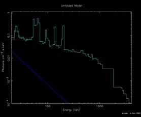 |
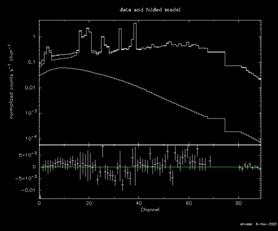
Note that without the "setplot group" command, XSPEC would plot 19 sets of spectral data, models and residuals. The can become confusing, especially as the number of spectra included in an analysis becomes much larger than 19! On the other hand, it can be useful to divide the data into subsets for plotting purposes, e.g. setplot group 1-6 7-12 13-19, to get an idea of relative shadowing effects of the coded-mask. The left hand plot illustrates the source model, the background model, the total model (i.e. source + background), and the data (here in count rates per channel). The right hand plot illustrates the "unfolded model" (blue, power-law curve), the summed model, and the data as a photon flux. A possible source of confusion is the similarity of the background model curves plotted in theses two separate representations. The explanation is that the background, which is dominated by instrumental contributions, is modeled in detector count space (i.e. the background response matrix has unit effective area. Thus, to be strictly correct, the right-hand plot is a hybrid of the photon source model and the detector-rate background model. We further note that at the present time, XSPEC does not have the capability to plot (or store and manipulate) the background subtracted data. This is a feature under consideration for a future release.
If we had chosen a observation containing more than a single source, the procedure would have been similar, except that the sequence of model commands would be extended, e.g.
XSPEC12>data ./MyDataDir/GCDE_aug_03.pha{1-475}
…
XSPEC12> model 1:1e1740 po
…
XSPEC12> model 2:gx1_4 po
…
XSPEC12> model 3:bkg spibkg_lo
…
Here data from the Galactic Center deep exposure campaign were loaded, and two sources are sought. In this case, a much larger number of spectra were loaded (475 spectra corresponds to one full 5´5 dither using all 19 detectors.
In this case, the simple approach of applying constant background (i.e. no detector-to-detector or pointing-to-pointing variation) to the full data set is likely to be a poor approximation. A more realistic approach would be to use the XSPEC grouping capability to handle such variations in the background solution. This can be accomplished in the usual manner (refer to the description of the grouping command in this document), however, it can become tedious in terms of the required command line inputs. For example, to establish a separate data group for each detector for a long (e.g. 5´5 dither) observations, a sequence of commands such as this would be required:
XSPEC12> data 1:1 ./MyDataDir/rev0044_Crab.pha.fits{1}
XSPEC12> data 2:2 ./MyDataDir/rev0044_Crab.pha.fits{2}
XSPEC12> data 3:3 ./MyDataDir/rev0044_Crab.pha.fits{3}
...
XSPEC12> data 19:19 ./MyDataDir/rev0044_Crab.pha.fits{19}
XSPEC12> data 1:20 ./MyDataDir/rev0044_Crab.pha.fits{20}
XSPEC12> data 2:21 ./MyDataDir/rev0044_Crab.pha.fits{21}
XSPEC12> data 3:22 ./MyDataDir/rev0044_Crab.pha.fits{22}
...
XSPEC12> data 19:38 ./MyDataDir/rev0044_Crab.pha.fits{38}
XSPEC12> data 1:39 /MyDataDir/rev0044_Crab.pha.fits{39}
XSPEC12> data 2:40 ./MyDataDir/rev0044_Crab.pha.fits{40}
XSPEC12> data 3:41 ./MyDataDir/rev0044_Crab.pha.fits{41}
...
XSPEC12> data 18:474 ./MyDataDir/rev0044_Crab.pha.fits{474}
XSPEC12> data 19:475 ./MyDataDir/rev0044_Crab.pha.fits{475}
One might then for example, make a first cut attempt by fitting a constant background. Then, as a next step, one might allow the normalization terms of the background model to vary over the groups (i.e. over the detector plane). This is accomplished with the "untie" command, using the following sequence:
XSPEC12> untie bkg:52
XSPEC12> untie bkg:78
XSPEC12> untie bkg:104
XSPEC12> untie bkg:130
XSPEC12> untie bkg:156
XSPEC12> untie bkg:182
XSPEC12> untie bkg:208
XSPEC12> untie bkg:234
XSPEC12> untie bkg:260
XSPEC12> untie bkg:286
XSPEC12> untie bkg:312
XSPEC12> untie bkg:338
XSPEC12> untie bkg:364
XSPEC12> untie bkg:390
XSPEC12> untie bkg:416
XSPEC12> untie bkg:442
XSPEC12> untie bkg:468
XSPEC12> untie bkg:487
Note that use of the "bkg" identifier, which associates the parameters index with the background model. The specific sequence of numbers use here requires some explanation; the particular background model employed has 25 parameters (which simply correspond in rank order to the 25 most variable individual bins), and a normalization term, i.e. parameter 26. Thus, the normalization for the second detector group is parameter 52, for the third parameter 78, and so on. Similar command sequences can be used to untie additional background model parameters. Supposing that we did this and refitted the data. We then might, for example wish to go back and freeze the individual normalization terms with the freeze command:
XSPEC12> freeze bkg:26
XSPEC12> freeze bkg:52
…
XSPEC12> freeze bkg:487
By now though, you probably get the idea that this all requires an unreasonable amount of command-line input. To circumvent this problem, a number of INTEGRAL/SPI specific "tcl" scripts are available which greatly streamline this process.
SPIdata
The SPIdata procedure, which when installed can be treated as an XSPEC command, greatly facilitates the data initialization step. For example, the command
XSPEC12> SPIdata ./MyData/Dir/rev0044_crab.pha 475 det Y
Opens the Crab observation spectral data file, reads the 475 spectra into memory, grouping them by detector. The "Y" then indicates that, yes, I wish to ignore the spectral data channels corresponding to the known detector-electronic noise contamination (this is the default). Instead of "det" as the grouping option I could have selected "time" to group by time (quantized into dither-pointing intervals). A "-" lead to the data being initialzed into a single group. The command:
XSPEC12> SPIdata ./MyData/Dir/rev0044_crab.pha 475
Reads the 475 spectra into a single data group, and ignores the undesirable channels. If you forget all this, the command
XSPEC12> SPIdata -h
will remind you. The scripts SPIuntie, and SPIfreeze have similar command-line syntax.
SPIuntie and SPIfreeze
XSPEC12> SPIuntie bkg 475 19 -1
The SPIuntie command script will accomplish the same result as the sequence of "untie" commands in the INTEGRAL/SPI example presented in this document. In that case, we had loaded 475 spectra associated with a single 5´5-dither pattern centered on the Crab nebula. The spectra were grouped by detector, which is a common approach to SPI analysis given the known detector-to-detector variations in the background rates. Suppose after an initial fitting pass, for which we assumed a single background spectrum, we know wish to untie the individual data group (i.e. detector) background models. This can be accomplished by issuing 25 "untie" commands as previously noted, or in a single command line using the SPIuntie command:
XSPEC12> SPIuntie bkg 475 19 -1
untie bkg:52
Chi-Squared = 1.2030200E+04 using 1615 PHA bins.
Reduced chi-squared = 7.5852458E+00 for 1586 degrees of freedom
Null hypothesis probability = 0.0000000E+00
untie bkg:78
Chi-Squared = 1.2030200E+04 using 1615 PHA bins.
Reduced chi-squared = 7.5900314E+00 for 1585 degrees of freedom
Null hypothesis probability = 0.0000000E+00
untie bkg:104
renorm: no renormalization necessary
Chi-Squared = 1.2030200E+04 using 1615 PHA bins.
Reduced chi-squared = 7.5948231E+00 for 1584 degrees of freedom
Null hypothesis probability = 0.0000000E+00
…
One might then make a second pass at fitting the data, hopefully leading to improved statistics. Subsequently, additional background model parameters could be untied using the SPIuntie procedure as well. For example, to untie three additional parameters over the full data set[1], the command syntax is:
XSPEC12> SPIuntie bkg 475 19 1 3
…
This will untie the first 3 parameters of the background model identified by "bkg", i.e. equivalent to issuing (475-1)´3 individual untie commands. Note that you can always be reminded of the command-line argument definitions by typing "SPIuntie -h" at the XSPEC prompt.
Suppose now that you are satisfied with the relative background normalization terms, and wish to freeze them at their current values for subsequent fitting passes. This could be accomplished using the SPIfreeze command script:
XSPEC12> SPIfreeze bkg 475 -1
XSPEC12>SPIfreeze bkg 19 1 -1
freeze bkg:52 1
Chi-Squared = 6.6232600E+05 using 1805 PHA bins.
Reduced chi-squared = 3.7589444E+02 for 1762 degrees of freedom
Null hypothesis probability = 0.0000000E+00
freeze bkg:78
Chi-Squared = 6.5791894E+05 using 1805 PHA bins.
Reduced chi-squared = 3.7318148E+02 for 1763 degrees of freedom
Null hypothesis probability = 0.0000000E+00
…
As with the SPIuntie command script, typing "SPIfreeze -h" at the XSPEC prompt will scroll the command-line definitions to your screen.
[1] Note that the current SPI background models, which are documented elsewhere, are designed so that the parameter list is hierarchically ordered in terms of decreasing criticality. Thus, freeing the first parameter is likely to have the most significant impact on the statistics, the second parameter, the next most significant, and so on.