Statistics in XSPEC

Introduction

There are two operations performed in XSPEC that require statistics. The first is parameter estimation, which comprises finding the parameters for a given model that provide the best fit to the data and then estimating uncertainties on these parameters. The second operation is testing whether the model and its best-fit parameters actually match the data. This is usually referred to as determining the goodness-of-fit.

Which statistics should be used for these two operations depends on the probability distributions underlying the data. Almost all astronomical data are drawn from one of two distributions: Gaussian (or normal) and Poisson. The Poisson distribution is the familiar case of counting statistics and is valid whenever the only source of experimental noise is due to the number of events arriving at the detector.  This is a good approximation for modern CCD instruments. If some other sort of noise is dominant then it is usually described by the Gaussian distribution. A common example of this is detectors that require background to be modeled in some way, rather than directly measured. The uncertainty in the background modeling is assumed to be Gaussian.

In the limit of large numbers of counts the Poisson distribution can be well approximated by a Gaussian so the latter is often used for detectors with high counting rates. In most cases this will cause no errors and does simplify the handling of background uncertainties however care should be exercised that no systematic offsets are introduced.

A fuller discussion of many of the issues discussed in this appendix can be found in Siemiginowska (2011).

Parameter Estimation

The standard statistic used in parameter estimation is the maximum likelihood. This is based on the intuitive idea that the best values of the parameters are those that maximize the probability of the observed data given the model. The likelihood is defined as the total probability of observing the data given the model and current parameters. In practice, the statistic used is twice the negative log likelihood.

For Gaussian data (chi)

The likelihood for Gaussian data is

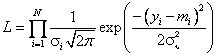
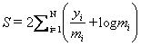
where y_i are the observed data rates, σ_i their errors, and m_i the values of the predicted data rates based on the model (with current parameters) and instrumental response. Taking twice the negative natural log of L and ignoring terms which depend only on the data (and will thus not change as parameters are varied) gives the familiar statistic :

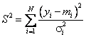
commonly referred to as χ² and used for the statistic chi option.

 

For Gaussian data with background (chi)

The previous section assumed that the only contribution to the observed data was from the model. In practice, there is usually background. This can either be included in the model or taken from another spectrum file (read in using the back command). In the latter case the y_i become observed data rates from the source spectrum subtracted by the background spectrum and the σ_i are the source and background errors added in quadrature. Since the difference of two Gaussians variables is another Gaussian variable, the S² statistic can still be used in this case.

For Poisson data (cstat)

The likelihood for Poisson distributed data is:

where S_i are the observed counts, t the exposure time, and m_i the predicted count rates based on the current model and instrumental response. The maximum likelihood-based statistic for Poisson data, given in Cash (1979), is :

Castor (priv. comm) has pointed out that modifying this by a quantity that depends only on the data (and hence makes no difference to the best-fit parameters) to give :

provides a statistic which asymptotes to S² in the limit of large number of counts. This is what is used for the statistic cstat option.

For Poisson data with Poisson background (cstat)

This case is more difficult than that of Gaussian data because the difference between two Poisson variables is not another Poisson variable so the background data cannot be subtracted from the source and used within the C statistic. The combined likelihood for the source and background observations can be written as:

 

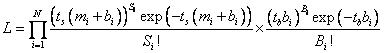
where t_s and t_b are the exposure times for the source and background spectra, respectively, B_i are the background data and b_i the predicted rates from a model for the expected background. If there is a physically motivated model for the background then this likelihood can be used to derive a statistic which can be minimized while varying the parameters for both the source and background models.

As a simple illustration suppose the source spectrum is source.pha and the background spectrum back.pha. The source model is an absorbed apec and the background model is a power-law. Further suppose that the background model requires a different response matrix to the source, backmod.rsp say. The fit is set up by:

XSPEC12> data 1:1 source.pha 2:2 background.pha

XSPEC12> resp 2:1 backmod.rsp 2:2 backmod.rsp

XSPEC12> model phabs(apec)

XSPEC12> model 2:backmodel pow

where the normalization of the apec model is fixed to zero for the second data group (i.e. the background spectrum) and the parameters of the background model are linked between the data groups.

If there is no appropriate model for the background it is still possible to proceed. Suppose that each bin in the background spectrum is given its own parameter so that the background model is b_i = f_i . A standard XSPEC fit for all these parameters would be impractical however there is an analytical solution for the best-fit f_i in terms of the other variables which can be derived by using the fact that the derivative of L will be zero at the best fit. Solving for the f_i  and substituting gives the profile likelihood:

where

and

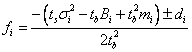
The sign of d_i in f_i is chosen so that f_i > 0. If any bin has S_i and/or  B_i  zero then its contribution to W (W_i) is calculated as a special case. So, if S_i  is zero then:

If B_i is zero then there are two special cases. If m_i < S_i / t_s then:

otherwise:

This W statistic is used for statistic cstat if a background spectrum with Poisson statistics has been read in. In practice, it works well for many cases but for weak sources can generate an obviously wrong best fit. It is not clear why this happens although binning to ensure that every bin contains at least one count often seems to fix the problem.

In the limit of large numbers of counts per spectrum bin a second-order Taylor expansion shows that W tends to :

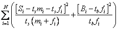
which is distributed as χ² with N – M degrees of freedom, where the model m_i has M parameters (include the normalization).

For Poisson data with Gaussian background (pgstat)

Another possible background option is if the background spectrum is not Poisson. For instance, it may have been generated by some model based on correlations between the background counts and spacecraft orbital position. In this case there may be an uncertainty associated with the background which is assumed to be Gaussian. In this case the same technique as above can be used to derive a profile likelihood statistic :

where

and

There is a special case for any bin with S_i  equal to zero:

 

This is what is used for the statistic pgstat option.

Bayesian analysis of Poisson data with Poisson background (lstat)

An alternative approach to fitting Poisson data with background is to use Bayesian methods. In this case instead of solving for the background rate parameters we marginalize over them writing the joint probability distribution of the source parameters as :

where {θ_j} are the source parameter, {b_k} the background rate parameters and I any prior information. Using Bayes theorem, that the {θ_j} and independent of the {b_k}, that the {b_k} are individually independent and that the observed counts are Poisson gives :

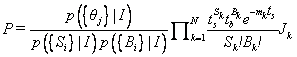
where :

To calculate J_k we need to make an assumption about the prior background probability distribution, p(b_k|I). We follow Loredo (1992) and assume a uniform prior between 0 and b_i^max. Expanding the binomial gives :

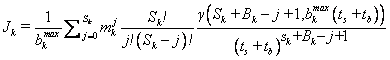
where :

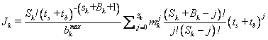
Again, follow Loredo we assume that and using the approximation when gives :

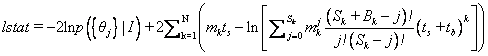
Note that for m_k = 0 only the j = 0 term in the summation is non-zero. Now, we define lstat by calculating -2 ln P and ignoring all additive terms which are independent of the model parameters :

For power spectra from time series data (whittle)

XSPEC has been used by a number of researchers to fit models to power spectra from time series data. In this case the x-axis is frequency (in Hz) and not keV so plots have to be modified appropriately. The correct fit statistic is that due to Whittle as discussed in Vaughan (2010) and Barret & Vaughan (2012) :

 

Parameter confidence regions

Fisher Matrix

XSPEC provides several different methods to estimate the precision with which parameters are determined.  The simplest, and least reliable, is based on the inverse of the second derivative of the statistic with respect to the parameter at the best fit. The first derivative must be zero by construction and the second derivative provides a measure of how rapidly the statistic increases away from the best-fit. The faster the statistic increases, i.e. the larger the second derivative, the more precisely the parameter is determined. The matrix of second derivatives is often referred to as the Fisher information. Its inverse is the covariance matrix, written out at the end of an XSPEC fit.

The +/- numbers provided for each parameter in the standard fit output are estimates of the one-sigma uncertainty, calculated as the square root of the diagonal elements of the covariance matrix. As such, these ignore any correlations between parameters. Whether correlations are important can be seen by comparing with the off-diagonal elements of the covariance matrix. In general, these estimates should be considered lower limits to the true uncertainty.

Correlation information is also given in the table of variances and principal axes which also appears at the end of a fit. Each row in this table is an eigenvalue and associated eigenvector of the Fisher matrix. If the parameters are independent then each eigenvector will have a contribution from only one parameter. For instance, if there are three independent parameters then the eigenvectors will be (1,0,0), (0,1,0), and (0,0,1). If the parameters are not independent then each eigenvector will show contributions from more than one parameter.

Delta Statistic

The next most reliable method for deriving parameter confidence regions is to find surfaces of constant delta statistic from the best-fit value, i.e. where :

This is the method used by the error command, which searches for the parameter value where the statistic differs from that at the best fit by a value (Δ) specified in the command. For each value of the parameter being tested all other free parameters are allowed to vary. The results of the error command can be checked using steppar, which can also be used to find simultaneous confidence regions of multiple parameters. The specific values of Δ which generate particular confidence regions are calculated by assuming thatis distributed as  χ² with the number of degrees of freedom equal to the number of parameters being tested (e.g. when using the error command there is one degree of freedom, when using steppar for two parameters followed by plot contour there are two degrees of freedom). This assumption is correct for the S² statistic and is asymptotically correct for other statistic choices.

Monte Carlo

The best but most computationally expensive methods for estimating parameter confidence regions are using two different Monte Carlo techniques. The first technique is to start with the best fit model and parameters and simulate datasets with identical properties (responses, exposure times, etc.) to those observed. For each simulation,  perform a fit and record the best-fit parameters.  The sets of best-fit parameters now map out the multi-dimensional probability distribution for the parameters assuming that the original best-fit parameters are the true ones. While this is unlikely to be true, the relative  distribution should still be accurate so can be used to estimate confidence regions. There is no explicit command in XSPEC to use this technique however it is easy to construct scripts to perform the simulations and store the results.

The second technique is Markov Chain Monte Carlo (MCMC) and is of much wider applicability. In MCMC a chain of sets of parameter values is generated which describe the parameter probability distribution. This determines both the best-fit (the mode) and the confidence regions. The chain command runs MCMC chains which can be converted to probability distributions using margin (which takes the same arguments as steppar). The results can be plotted in 1- or 2-D using plot margin however this is not quite as useful as it might be because what is plotted is the probability, not the probability within some region. If MCMC chains are in use then the error command will use them to estimate the parameter uncertainty.

 

Goodness-of-fit

Parameter values and confidence regions only mean anything if the model actual fits the data. The standard way of assessing this is to perform a test to reject the null hypothesis that the observed data are drawn from the model. Thus we calculate some statistic T and if T_obs > T_critical then we reject the model at the confidence level corresponding to T_critical. Ideally, T_critical is independent of the model so all that is required to evaluate the test is a table giving T_critical values for different confidence levels. This is the case for χ² which is one of the reasons why it is used so widely. However, for other test statistics this may not be true and the distribution of T must be estimated for the model in use then the observed value compared to that distribution. This is done in XSPEC using the goodness command. The model is simulated many times and a value of T calculated for each fake dataset. These are then ordered and a distribution constructed. This distribution can be plotted using plot goodness. Now suppose that T_obs exceeds 90% of the simulated T values, we can reject the model at 90% confidence.

It is worth emphasizing that goodness-of-fit testing only allows us to reject a model with a certain level of confidence, it never provides us with a probability that this is the correct model.

Chi-square (chi)

The standard goodness-of-fit test for Gaussian data is χ² (as defined above). At the end of a fit, XSPEC writes out the reduced χ² (= χ²/ν , where ν is the number of degrees of freedom = number of data bins – number of free parameters). A rough rule of thumb is that the reduced χ² should be approximately one.  If the reduced χ² is much greater than one then the observed data are likely not drawn from the model. If the reduced χ² is much less than one then the Gaussian sigma associated with the data are likely over-estimated. XSPEC also writes out the null hypothesis probability, which is the probability of the observed data being drawn from the model given the value of  χ² and the number of degrees of freedom.

Pearson chi-square (pchi)

Pearson's original (1900) chi-square test was not for Gaussian data but for the case of dividing counts up between cells. This corresponds to the case of Poisson data with no background.

Kolmogorov-Smirnov (ks)

There are a number of test statistics based on the empirical distribution function (EDF). The EDF is the cumulative spectrum :

and  

The EDF can be plotted using plot icounts. The best known of these tests is Kolmogorov-Smirnov whose statistic is simply the largest difference between the observed and model EDFs :

The XSPEC statistic test ks option returns log D. The significance of the ks value can be determined using the goodness command.

Cramer-von Mises (cvm)

The Cramer-von Mises statistic is the sum of the squared differences of the EDFs :

The XSPEC statistic test cvm option returns log w² and its significance should be determined using the goodness command.

Anderson-Darling (ad)

Anderson-Darling is a modification of Cramer-von Mises which places more weight on the tails of distribution :

Runs (runs)

The Runs (or Wald-Wolfowitz) test checks that residuals are randomly distributed above and below zero and do not cluster. Suppose N_p is the number of channels with +ve residuals, N_n the number of channels with negative residuals, and R the number of runs then the Runs statistic is :

where :

and

As for the EDF tests, XSPEC returns log Runs.

 

References

Barret, D. & Vaughan, S., 2012. “Maximum likelihood fitting of X-ray power density spectra: application to high-frequency quasi-periodic oscillation from the neutron star X-ray binary 4U1608-522”, ApJ 746, 131.

Cash, W., 1979. “Parameter estimation in astronomy through application of the likelihood ratio”,  ApJ 228, 939.

Loredo, T., 1992. In “Statistical Challenges in Modern Astronomy”, eds. Feigelson, E.D. and Babu, G.J., pp 275-297.

Siemiginowska, A., 2011. In “Handbook of X-ray Astronomy” eds. Arnaud, K.A., Smith, R.K. and Siemiginowska, A., Cambridge University Press, Cambridge.

Vaughan, S. 2010, “A Bayesian test for periodic signals in red noise”, MNRAS 402, 307.